반응형
결정 트리의 앙상블 - 랜덤 포레스트
- 앙상블 ensemble은 여러 머신러닝 모델을 연결하여 더 강력한 모델을 만드는 기법
- 랜덤 포레스트 random forest, 그래디언트 부스팅 gradient boosting 결정 트리는 둘 다 모델을 구성하는 기본 요소로 결정 트리를 사용
- 결정 트리의 주요 단점은 훈련 데이터에 과대 적합이 되는 경향 → 랜덤 포레스트는 이 문제를 회피할 수 있는 방법
- 랜덤 포레스트 아이디어
- 각 트리는 비교적 예측을 잘 할 수 있지만 데이터의 일부에 과대 적합하는 경향을 가진다는데 기초
- 잘 작동하되 서로 다른 방향으로 과대적합된 트리를 많이 만들면 그 결과를 평균냄으로써 과대적합된 양을 줄임
- 트리 모델의 예측 성능이 유지되면서 과대적합이 줄어드는 것이 수학적으로 증명
- 랜덤 포레스트는 이름에서 알 수 있듯이 트리들이 달라지도록 트리 생성 시 무작위성을 주입
- 랜덤 포레스트에서 트리를 랜덤하게 만드는 방법은 두 가지
- 트리를 만들 때 사용하는 데이터 포인트를 무작위로 선택하는 방법
- 분할 테스트에서 특성을 무작위로 선택하는 방법
결정 트리의 앙상블 - 랜덤 포레스트 구축
- 랜덤 포레스트 모델을 만들려면 생성할 트리의 개수를 정해야함
- RandomForestRegressor 나 RandomForestClassifier의 n_estimators 매개변수 설정
- 트리를 만들기 위해 먼저 데이터의 부트스트랩 샘플 (bootstrap sample)을 생성
- n_samples개의 데이터 포인트 중에서 무작위로 데이터를 n_samples 횟수만큼 반복 추출
- 이렇게 만든 데이터셋으로 결정 트리를 만듬
- 각 노드에서 특성의 일부만 사용하기 때문에 트리의 각분기는 각기 다른 특성 부분 집합을 사용
- 핵심 매개변수는 max_features - max_features=1로 설정하면 트리의 분기는 테스트할 특성을 고를 필요가 없게 되며 그냥 무작위로 선택한 특성의 임계값을 찾음
- 결국 max_features 값을 크게 하면 랜덤 포레스트의 트리들은 매우 비슷해지고 가장 두드러진 특성을 이용해 데이터에 잘 맞춰질 것
- 회귀와 분류에 있어서 랜덤 포레스트는 현재 가장 널리 사용되는 머신러닝 알고리즘
- 유념할 점은 랜덤 포레스트는 이름 그대로 랜덤
- 랜덤 포레스트는 텍스트 데이터 값이 매우 차원이 높고 희소한 데이터에는 잘 작동하지 않음
결정 트리 앙상블 - 그래디언트 부스팅 회귀 트리
- 그래디언트 부스팅 회귀 트리는 여러 개의 결정 트리를 묶어 강력한 모델을 만드는 또 다른 앙상블 방법
- 이전 트리의 오차를 보완하는 방식으로 순차적으로 트리를 만듬
- 기본적으로 그래디언트 부스팅 회귀 트리에는 무작위성이 없음 → 대신 강력한 사전 가지치기가 사용
- 그래디언트 부스팅 트리는 보통 하나에서 다섯 정도의 깊지 않은 트리를 사용하므로 메모리를 적게 사용하고 예측도 빠름
- scikit-learn에 구현된 GradientBoostingClassifier 사용
- 그래디언트 부스팅의 근본 아이디어
- 얕은 트리 같은 간단한 모델(약한 학습기 weak learnner라고도 함) 을 많이 연결하는 것
- 각각의 트리는 데이터의 일부에 대해서만 예측을 잘 수행할 수 있어서 트리가 많이 추가될수록 성능이 좋아짐
- 그래디언트 부스팅 트리는 머신러닝 경연 대회에서 우승을 많이 차지하였고 업계에서도 널리 사용
- 랜덤 포레스트보다는 매개변수 설정에 조금 더 민감하지만 잘 조정하면 더 높은 정확도를 제공
- 중요한 매개변수는 이전 트리의 오차를 얼마나 강하게 보정할 것인지를 제어하는 learning_rate
- 학습률이 크면 트리는 보정을 강하게 하기 때문에 복잡한 모델을 만듦
- n_estimators 값을 키우면 앙상블에 트리가 더 많이 추가되어 모델의 복잡도가 커지고 훈련 세틍에서의 실수를 바로잡을 기회가 더 많아짐
Ensemble Modeling Heart Disease 분류 모델 비교
문제 정의 : 환자 정보를 사용하여 심장 질환 유무 (정상:0, 심장 질환 진단 :1)를 예측하는 이진 분류 문제로 정의
데이터 다운로드 : https://archive.ics.uci.edu/ml/datasets/heart+disease
UCI Machine Learning Repository: Heart Disease Data Set
Heart Disease Data Set Download: Data Folder, Data Set Description Abstract: 4 databases: Cleveland, Hungary, Switzerland, and the VA Long Beach Data Set Characteristics: Multivariate Number of Instances: 303 Area: Life Attribute Characteristics: Categ
archive.ics.uci.edu
기본 라이브러리 임포트
import numpy as np
import pandas as pd

import matplotlib.pyplot as plt
import seaborn as sns
import plotly.express as px

from sklearn.model_selection import train_test_split
from sklearn.preprocessing import StandardScaler

from sklearn.linear_model import LogisticRegression
from sklearn.tree import DecisionTreeClassifier
from sklearn.ensemble import RandomForestClassifier
from sklearn.ensemble import GradientBoostingClassifier

from sklearn import metrics
데이터 준비하기
df = pd.read_csv('/content/heart.csv')
df.head()
df.info()
df.isna().sum()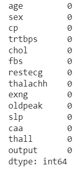
df.isnull().sum()
데이터 전처리
df['sex'].unique()
# 범주형 숫자가 아니라 onehot 인코딩으로 비교할 수 있게 만드는 것이 좋음
df['cp'].unique()
# chest pain 가슴 통증 강도를 의미하는 column
df['fbs'].unique()
# 얘도 범주형이네
df['restecg'].unique()
# 1) 카테고리(범주형) 변수 컬럼 -> onehot encoding
categorical_var = ['sex', 'cp', 'fbs', 'restecg', 'exng', 'slp', 'caa','thall']
df[categorical_var] = df[categorical_var].astype('category')
df.info()
# 2) 숫자형(연속형) 컬럼 -> 정규화
numberic_var = [i for i in df.columns if i not in categorical_var][:-1]

numberic_var
데이터 분석
sns.countplot(df.sex) # (1 = male; 0 = female)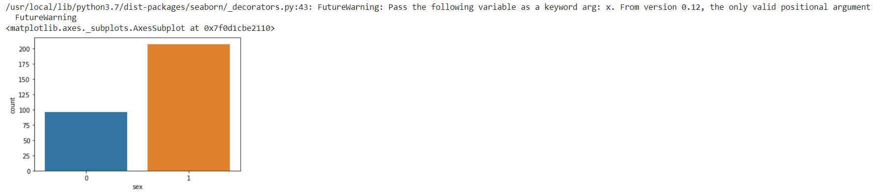
px.bar(df.groupby('cp').sum().reset_index()[['cp', 'output']], x='cp', y='output', color='cp')
df.groupby('cp').sum().reset_index()[['cp', 'output']]
df.output.value_counts().plot.pie(autopct='%1.f%%')
plt.show()
df.output.value_counts().plot.bar()
plt.show()
# 범주형 변수 (categorical_var)와 output(y) 관계를 시각화
fig, ax = plt.subplots(2,4,figsize=(10,5), dpi=200)

for axis, cat_var in zip(ax.ravel(), categorical_var):
  sns.countplot(x=cat_var, data=df, hue='output', ax=axis)

plt.tight_layout()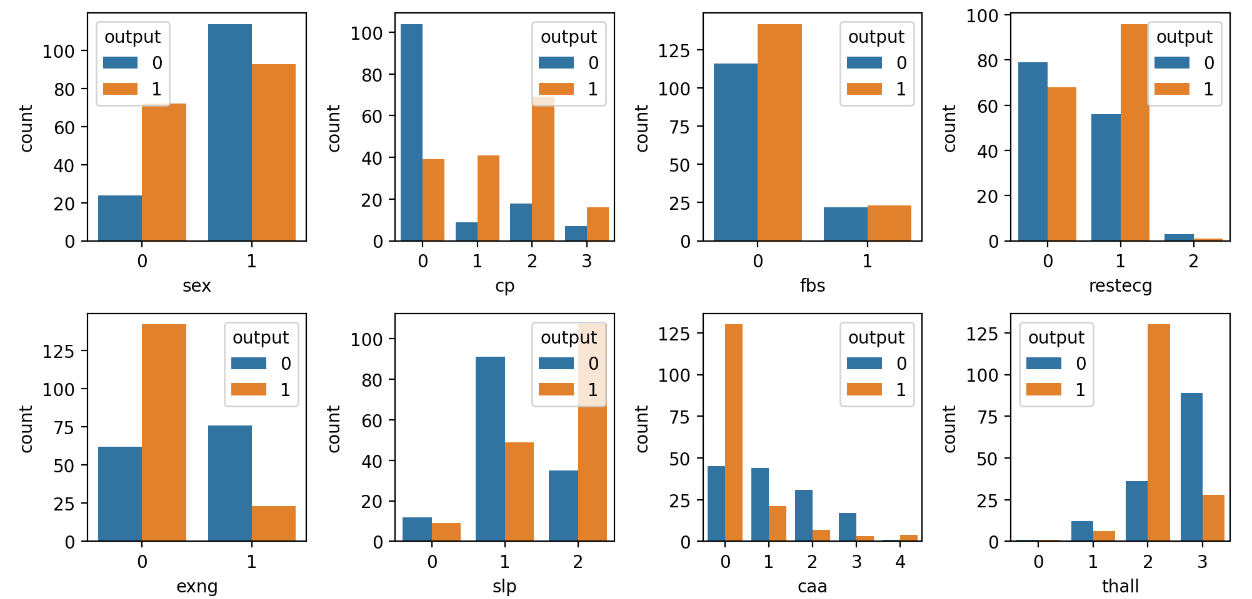
# 수치형(numberic_var)와 output(y)과의 관계 시각화

fig, ax = plt.subplots(1,5, figsize=(15,5), dpi=200)

for axis, num_var in zip(ax, numberic_var):
  sns.boxplot(y=num_var, data=df, x='output', ax=axis)

plt.tight_layout()
# 그래프 위 아래는 outlayer 이상치들임
# 정규화하기 전에 이상치들을 없애자.(정규화할 때도 이상치들 때문에 잘 안됨)
# 수치형 (numberic_var) 컬럼 중 나이 컬럼을 제외하고 5%의 이상치를 제거

# 상위 5%의 이상치를 삭제
df = df[df['trtbps'] < df['trtbps'].quantile(0.95)]
df = df[df['chol'] < df['chol'].quantile(0.95)]
df = df[df['oldpeak'] < df['oldpeak'].quantile(0.95)]

# 하위 5%의 이상치를 삭제
df = df[df['thalachh'] > df['thalachh'].quantile(0.05)]
fig, ax = plt.subplots(1,5, figsize=(15,5), dpi=200)
for axis, num_var in zip(ax, numberic_var): # zip을 통해서 한번에 두 변수에 두가지 range를 넘겨줄 수 있음
sns.boxplot(y=num_var, data=df, x='output', ax=axis)
plt.tight_layout()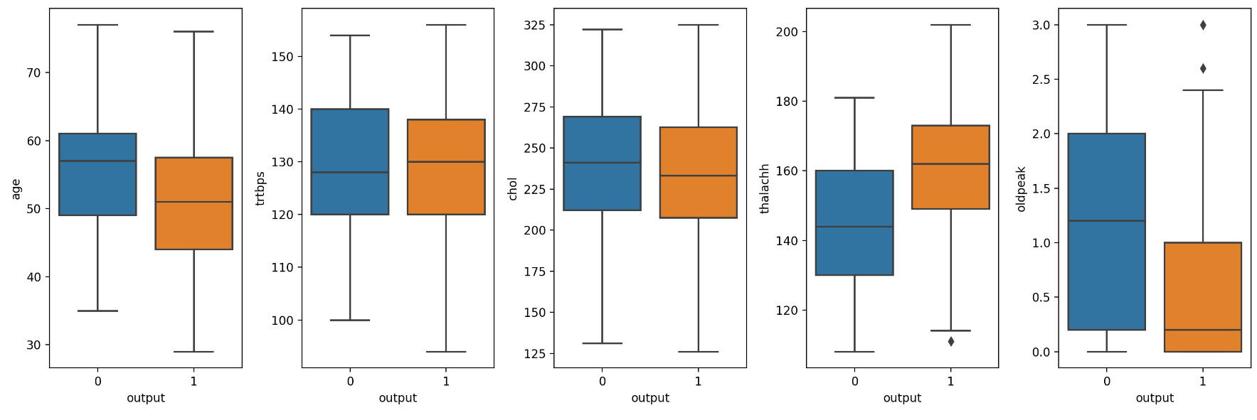
df.info()
데이터 분리하기
X = df.iloc[:, :-1]
y = df['output']
X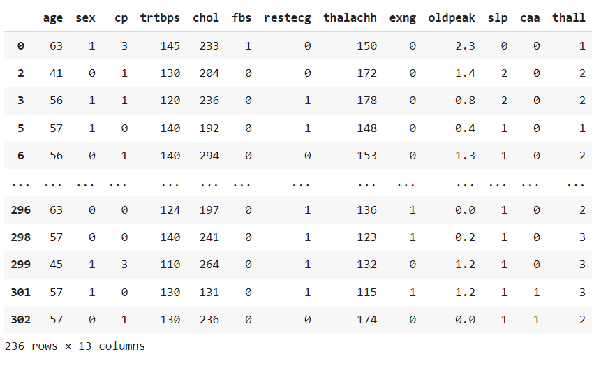
# 범주형 -> 원핫인코딩
temp_x = pd.get_dummies(X[categorical_var])

# 원핫 인코딩 컬럼 추가
X_modified = pd.concat([X,temp_x], axis=1)

# 기존 컬럼 삭제
X_modified.drop(categorical_var, axis=1, inplace=True)
X_modified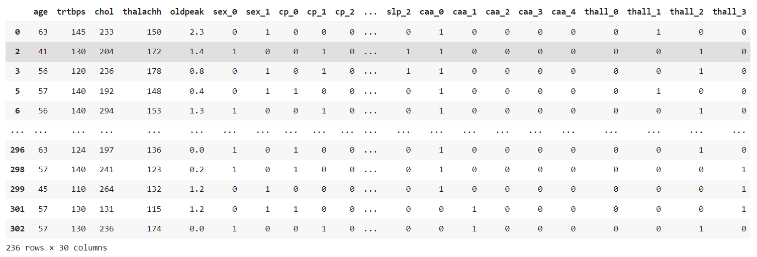
# 수치형 변수 -> 정규화 -> 스케일링
X_modified[numberic_var] = StandardScaler().fit_transform(X_modified[numberic_var])
X_modified.head()
Train, Test 데이터 분리하기
# 80:20 비율로 분리
X_train, X_test, y_train, y_test = train_test_split(X_modified, y, test_size=0.2, random_state=7)
X_train.shape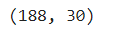
X_test.shape
머신러닝 모델 설정 및 학습
# 1. LogistricRegression
log_reg = LogisticRegression(C=0.04).fit(X_train, y_train)

print('훈련 세트 점수 : {:.5f}%'.format(log_reg.score(X_train, y_train)*100))
print('테스트 세트 점수 : {:.5f}%'.format(log_reg.score(X_test, y_test)*100))
# 2. DecisionTree
tree = DecisionTreeClassifier(max_depth=5, min_samples_leaf=20, min_samples_split=40).fit(X_train, y_train)

print('훈련 세트 점수 : {:5f}%'.format(tree.score(X_train, y_train)*100))
print('테스트 세트 점수 : {:.5f}%'.format(tree.score(X_test, y_test)*100))
# 3. RandomForest
random = RandomForestClassifier(n_estimators=9, random_state=7).fit(X_train, y_train)

print('훈련 세트 점수 : {:.5f}%'.format(random.score(X_train, y_train)*100))
print('테스트 세트 점수 : {:.5f}%'.format(random.score(X_test, y_test)*100))
# 4. GradientBoosting
boost = GradientBoostingClassifier(max_depth=3, learning_rate=0.034).fit(X_train, y_train)

print('훈련 세트 점수 : {:.5f}%'.format(boost.score(X_train, y_train)*100))
print('테스트 세트 점수 : {:.5f}%'.format(boost.score(X_test, y_test)*100))
train_scores = []
test_scores = []

rate = np.arange(0.033, 0.035, 0.001)

for r in rate:
  boost = GradientBoostingClassifier(max_depth=3, learning_rate=r).fit(X_train, y_train)

  train_scores.append(boost.score(X_train, y_train))

  test_scores.append(boost.score(X_test, y_test))
plt.figure(dpi=100)

plt.plot(rate, train_scores, label='train')
plt.plot(rate, test_scores, label='test')

plt.legend()
plt.show()
LIST
'대외활동 > ABC 지역주도형 청년 취업역량강화 ESG 지원산업' 카테고리의 다른 글
| [ABC 220926] 특강 "야나두 할 수 있는 재무설계" (0) | 2022.10.20 |
|---|---|
| [ABC 220923] 지도 학습 알고리즘 - 요약 및 정리 (0) | 2022.10.20 |
| [ABC 220923] 지도 학습 알고리즘 - 결정 트리 (1) | 2022.10.18 |
| [ABC 220923] 지도 학습 알고리즘 - 선형 모델 정리 (1) | 2022.10.18 |
| [ABC 220923] 지도 학습 알고리즘 - 서포트 벡터 머신 (0) | 2022.10.18 |

