반응형
당뇨병 발병 유무 예측
문제 정의하기
- 이진 분류 예제에 적합한 데이터셋은 8개 변수와 당뇨병 발병 유무가 기록된 '피마족 인디언 당뇨병 발병 데이터셋'
- 8개의 변수를 독립변수로 보고 당뇨병 발병 유무를 예측하는 이진 분류 문제로 정의(결과로 1이면 당뇨병, 0이면 아님)
데이터 준비하기
- http://www.kaggle.com/uciml/pima-indians-diabetes-database
- 8가지 속성 (1번 ~ 8번)과 결과(9번)
- 임신 횟수
- 경구 포도당 내성 검사에서 2시간 동안의 혈장 포도당 농도
- 이완기 혈압 (mm Hg)
- 삼두근 피부 두겹 두께 (mm)
- 2 시간 혈청 인슐린 (mu U/ml)
- 체질량 지수
- 당뇨 직계 가족력
- 나이 (세)
- 5년 이내 당뇨병이 발병 여부
데이터셋 생성하기
- 입력(속성값 8개)와 출력(판정결과 1개) 변수 70:30 비율, 학습 데이터 : 614건, 테스트 데이터 : 154건 → 총 데이터 768건
모델 구성하기
- Dense 레이어만을 사용하여 다층 퍼셉트론 모델을 구성 데이터 준비하기
- 속성이 8개이기 때문에 입력 뉴런은 8개이고, 이진 분류이기 때문에 0~1 사이의 값을 나타내는 출력 뉴런이 1개
- 출력 레이어만 0과 1사이로 값이 출력될 수 있도록 활성화 함수를 'sigmoid'로 사용
model = Sequential()
model.add(Dense(12, input_dim=8, activation='relu')
model.add(Dense(8, activation='relu'))
model.add(Dense(1, activation='sigmoid'))
모델 학습 과정 설정하기
- 모델을 정의했다면 모델을 손실함수와 최적화 알고리즘(하이퍼파라미터) 설정
- loss : 이진 클래스 문제이므로 'binary_crossentropy'으로 지정
- optimizer : 효율적인 경사 하강법 알고리즘 중 하나인 'adam'을 사용
- metrics : 평가 척도를 나타내며 분류 문제에서는 일반적으로 'accuracy'로 지정
model.compile(loss='binary_crossentropy', optimizer='adam', metrics=['accuracy'])모델 학습시키기
- 모델을 학습시키기 위해서 fit() 함수를 사용
- 첫번째 인자 : 8개의 속성 값을 담고 있는 X(입력변수)를 입력
- 두번째 인자 : 라벨값(정답) 결과를 담고 있는 Y(출력변수)를 입력
- epochs : 전체 훈련 데이터셋에 대해 학습 반복 횟수를 지정(1000번을 반복적으로 학습)
- batch_size : 가중치를 업데이트할 배치 크기를 의미하며, 128개로 지정
history = model.fit(X_train, y_train, epochs=1500, batch_size=128)모델 평가하기
- 테스트 셋으로 학습한 모델을 평가
scores = model.evaluate(X_test, y_test)
print("%s : %.2f%%" %(model.metrics_names[1], scores[1]*100))
실습하기
데이터 준비하기
import pandas as pd
import numpy as np
from sklearn.model_selection import train_test_split

import tensorflow as tf
from keras.models import Sequential
from keras.layers import Dense

# 랜덤 시드 고정
np.random.seed(5)
dataset = pd.read_csv('/content/diabetes.csv')
dataset.head()
데이터 확인하기
dataset.info()
데이터 분리하기
dataset.columns
X = dataset[['Pregnancies', 'Glucose', 'BloodPressure', 'SkinThickness', 'Insulin',
       'BMI', 'DiabetesPedigreeFunction', 'Age']]
y = dataset['Outcome']

# train:test = 80:20 => 614:154
X_train, X_test, y_train, y_test = train_test_spilt(X, y, test_size=02, random_state=777)
X_train.shape
모델 구성하기
model = Sequential()
model.add(Dense(32, input_dim=8, activation='relu'))
model.add(Dense(8, activation='relu'))
model.add(Dense(1, activation='sigmoid'))
model.summary()
tf.keras.utils.plot_model(model, show_shapes=True, show_layer_names=True, rankdir='TB', expand_nested=False, dpi=100)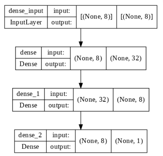
모델 설정하기
model.compile(loss='binary_crossentropy', optimizer='adam', metrics=['accuracy'])모델 학습하기
history = model.fit(X_train, y_train, epochs=100, batch_size=128)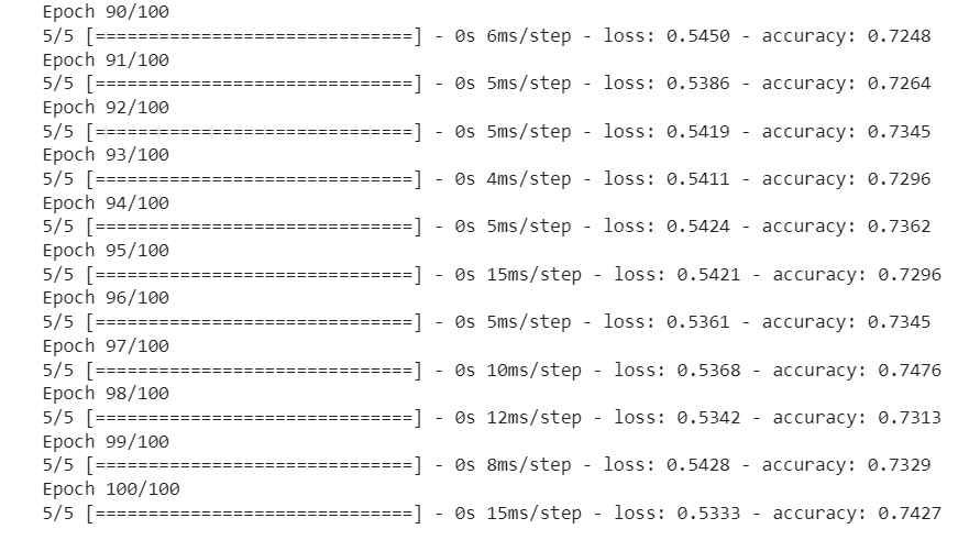
학습결과
import matplotlib.pyplot as plt

his_dixt = history.history
loss = his_dict['loss']

epochs = range(1, len(loss) + 1)
fig = plt.figure(figsize=(10,5))

# 훈련 및 검증 손실 그리기
ax1 = fig.add_subplot(1, 2, 1)
ax1.plot(epochs, loss, color = 'orange', label = 'train_loss')
ax1.set_title('train loss')
ax1.set_xlabel('epochs')
ax1.set_ylabel('loss')
ax1.legend()

acc = his_dict['accuracy']

# 훈련 및 검증 정확도 그리기
ax2 = fig.add_subplot(1, 2, 2)
ax2.plot(epochs, acc, color = 'blue', label = 'train_accuracy')
ax2.set_title('train accuracy')
ax2.set_xlabel('epochs')
ax2.set_ylabel('accuracy')
ax2.legend()

plt.show()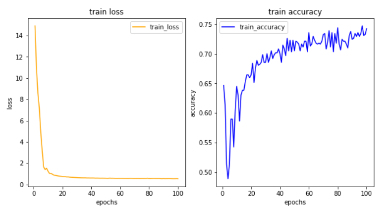
모델 평가하기
scores = model.evaluate(X_test, y_test)
print('%s : %.2f%%' %(model.metrics_names[1], score[1]*100))
print(model.metrics_names[0], score[0])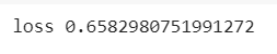
scores = model.evaluate(X_train, y_train)
print('%s: %.2%%' %(model.metrics_names[1], scores[1]*100))
반응형
'대외활동 > ABC 지역주도형 청년 취업역량강화 ESG 지원산업' 카테고리의 다른 글
| [220928 ABC] 피마족 인디언 당뇨병 발병 유무 예측(정규화 추가 ver) (0) | 2022.12.05 |
|---|---|
| [220928 ABC] 신경망과 케라스 정리 (0) | 2022.10.30 |
| [220928 ABC] 케라스에서의 개발 과정 (1) | 2022.10.30 |
| [220928 ABC] 신경망의 기본 개념 (1) | 2022.10.29 |
| [ABC 220927] 신경망 (0) | 2022.10.24 |


